Formal Verification

Testing is a kind of inductive reasoning to accumulate evidence in support of a conclusion but not validate the conclusion (the correctness of program) directly. (This “inductive” is different from the rigorous induction proof technique) Deductive reasoning proceeds from premises and rules about logic and go to a valid conclusion.

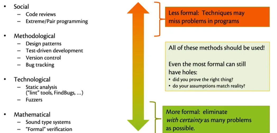
Formal verification is the task for proving that the implementation of the function satisfies its specification (from Chapter6 Video21)… It’s difficult to do that in an imperative language, because those expressions might have side effects that change the state.

Equational Reasoning

• based on equality between expressions
• to verify whether two pieces of code are equal semantically
• expressions, which are differnent in syntactics, evaluate to the sam value
• functions, when provided with the same input, produce the same output

Structural induction

Claim: forall n, P(n)
Proof: by induction on n

Base case: n = 0
Show: P(0)

Inductive case: n = k+1
IH: P(k)
Show: P(k+1)

QED

Write an obviously correct implementation that is lacking in some desired property, such as efficiency, then prove that a better implementation is equal to the original.

For example the textbook gives an example of prove the equivalence of factorial with and without tail recursion. (try to show forall p, p * fact n = facti p n)

The tail-recursive version is called iterative because it “strongly resembles how the same computation would be expressed using a loop” iteratively. Nice English tips, so I copied here.

And here is a formal proof on f_r = f_tr with or without tail recursion (recursive or iterative)

(* let rec f_r n =
  if n = 0 then i else op n (f_r (n - 1)) *)

Fixpoint f_r n :=
  match n with
  | 0 => 1
  | S n' => n * (f_r n')
  end.

(* let rec f_i acc n =
  if n = 0 then acc
  else f_i (op acc n) (n - 1)

let f_tr = f_i i *)
Fixpoint f_i acc n :=
  match n with
  | 0 => acc
  | S n' => f_i (acc * n) n'
  end.
Definition f_tr n := f_i 1 n.

Require Import Lia.

Lemma f_r_eq_f_i : forall n acc, acc * f_r n = f_i acc n.
Proof.
  induction n as [| n' IH].
  - simpl. lia.
  - simpl. intros.
    rewrite <- IH.
    lia.
Qed.

Lemma f_r_eq_f_tr : forall n, f_r n = f_tr n.
Proof.
  intros.
  unfold f_tr.
  rewrite <- f_r_eq_f_i with (acc := 1).
  simpl. lia.
Qed.

• partial correctness: meaning that if a program terminates, then its output is correct; and
• total correctness: meaning that a program does terminate, and its output is correct.

A Turing machine cannot decide whether a program halts, but SMART human sometimes do (how smart). A recursive function terminates if all its recursive calls are on elements that are smaller according to <, where < means descents and forms a “well-founded relation”.

Require Import List.
Import ListNotations.
Check app_assoc.

Lemma app_assoc' : forall (A : Type) (l1 l2 l3 : list A),
  l1 ++ (l2 ++ l3) = (l1 ++ l2) ++ l3.
Proof.
  intros A l1 l2 l3.
  induction l1 as [| x l1' IH].
  - simpl. reflexivity.
  - simpl. rewrite IH. reflexivity.
Qed.

Primitive recursive function

Primitive recursive function, intuitively, is a function that can be computed by a computer with for loops (instead of real while loops whose number of iterations of every loop cannot be decided before entering the loop)

Most computable functions are primitive recursive, like factorial. (Computabilty: can be computed by an algorithm with respect to a specific computation model) Formally, a function $f:\mathbb{N}^k \to \mathbb{N}$ is called primitive recursive if it belongs to the smallest class of functions that contains the basic functions below and is closed under the two operations below.

Basic functions are (using superscript to mean $k$-ary)

• the zero function $C^k_n(x_1,\dots,x_k)=0$
• the successor function $S(x)=x+1$
• and the projection functions $P_i^k(x_1,\dots,x_k)=x_i$ The closure operations are composition and primitive recursion
• (composition) if $g_1,\dots,g_m$ and $h$ are primitive recursive, then the function $f(\vec{x}) = h(g_1(\vec{x}),\dots,g_m(\vec{x}))$ is also primitive recursive.
• (primitive recursion) if $g(\vec{x})$ and $h(y,z,\vec{x})$ are primitive recursive, then the function $f$ defined by $f(0,\vec{x})=g(\vec{x})$ and $f(y+1,\vec{x})=h(y,f(y,\vec{x}),\vec{x})$ is also primitive recursive.

It’s clear to be a recursion scheme where each step for input $y+1$ is computed from the previous value at $y$, and $f$ acts as a for-loopfrom 0 up to the value of its first argument. Therefore, any primitive recursive function can be computed by applying these two rules only finitely many times, and then finally becomes evaluating the basic ones. Here are some interesting examples about how to write common computation as standard primitive recursive form.

Computable function

In computability theory, the μ-operator, minimization operator, or unbounded search operator searches for the least natural number with a given property. Adding the $\mu$-operator to the primitive recursive functions makes it possible to define all computable functions. (from wikipedia)

The complexity class $\textbf {PR}$ is languages that can be decided in time bounded by primitive functions. But there are recursive functions that are computable (like, by a TM) but not premitive recursive, so $\textbf{PR}\subsetneq \textbf R$, where $\textbf R$ is the class of all decision problems solvable by a TM (recursive/decidable languages).

let rec ack = function
  | (0, n) -> n + 1
  | (m, 0) -> ack (m - 1, 1)
  | (m, n) -> ack (m - 1, ack (m, n - 1))